
August 11, 2026
The Equation That Most Investors Never Finish Reading
Inflation analysis has a blind spot. It is not hidden in obscure academic literature or buried in central bank footnotes. It sits in plain sight inside one of the most fundamental identities in macroeconomics, a formula that most financial commentators quote incompletely and then abandon halfway through.
The equation of exchange, expressed as MV = PQ, connects the money supply to the price level through two monetary inputs, not one. M represents the money supply. V represents velocity, the rate at which money circulates. P is the aggregate price level. Q is real economic output. Every serious inflation forecast requires all four variables. Most mainstream commentary uses only one of them.
This structural gap in popular monetary analysis is not merely an academic oversight. It has real consequences for investors attempting to understand when and why monetary expansion produces price inflation, and what role assets like gold play in protecting purchasing power when the equation finally rebalances.
Understanding the relationship between the velocity of money and gold inflation is not a niche concern. It is one of the most practically important frameworks available to long-term investors operating in an era of historically elevated money supply.
When big ASX news breaks, our subscribers know first
Velocity: The Variable That Determines Whether Money Printing Matters
What Velocity Actually Measures
Velocity of money is the frequency with which each unit of currency in the M2 money supply finances economic transactions over a defined period. The Federal Reserve Bank of St. Louis calculates and publishes this metric quarterly on its FRED database under the series M2V, using a straightforward formula derived directly from the equation of exchange.
| Metric | Formula | Data Source |
|---|---|---|
| M2 Velocity (V) | Nominal GDP ÷ M2 Money Supply | FRED (M2V series) |
| Nominal GDP | Price Level × Real Output | Bureau of Economic Analysis |
| M2 Money Stock | Broad money aggregate | Federal Reserve |
To illustrate with current figures: if M2 equals approximately $22 trillion and annual nominal GDP equals approximately $31 trillion, velocity calculates to roughly 1.41. This means each dollar in the money supply financed about $1.41 of economic activity during that period. That figure is simultaneously revealing and alarming when placed in historical context.
High velocity reflects an economy where money moves rapidly and continuously through productive channels: from businesses paying wages, to employees purchasing goods, to suppliers receiving payment and reinvesting in production. Low velocity reflects the opposite condition — money accumulating in savings deposits, financial institution reserves, and money market instruments rather than financing real-world transactions.
Why the Multiplier Logic Changes Everything
The equation of exchange is not a theory or a model. It is an accounting identity. Given any three known variables, the fourth is mathematically determined. This has a critical implication that most inflation narratives ignore entirely: a doubling of the money supply combined with a simultaneous halving of velocity produces no net inflationary pressure on the price level, assuming real output remains stable.
Furthermore, as research from ScienceDirect on the velocity of money confirms, this relationship underpins much of modern monetary theory and yet remains routinely overlooked in mainstream economic commentary.
Core Framework: Inflation is the product of monetary volume multiplied by monetary circulation speed. Analysing M alone, without V, is like measuring the size of a reservoir without accounting for whether the floodgates are open or closed.
This is not a theoretical abstraction. It describes precisely what occurred in the United States between 2020 and 2022, with measurable consequences that followed a predictable sequence once velocity began recovering.
Six Decades of Velocity Data: A Regime Analysis
The Stable Era and Its Peak (1959 to 1997)
From the late 1950s through the mid-1990s, M2 velocity maintained a relatively consistent range of approximately 1.65 to 1.90, reflecting an economy where consumer spending, business investment, and credit expansion kept money circulating at a stable pace. This range represented what might be described as the baseline operating condition of a normally functioning monetary economy.
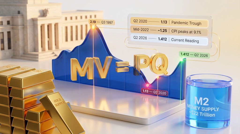
The dot-com era expansion broke that pattern decisively upward. Consumer confidence surged, corporate investment accelerated, and credit availability expanded rapidly. Velocity reached its all-time recorded peak of 2.19 in Q3 1997 according to FRED data. At that level, every dollar in M2 was financing more than $2.19 of nominal economic activity annually, reflecting an economy operating at maximum monetary efficiency.
The Three-Decade Structural Decline (1997 to 2020)
Following the 1997 peak, velocity entered a prolonged structural downtrend spanning nearly 23 years. This was not cyclical volatility. The decline was continuous, consistent, and driven by interlocking structural forces that each reinforced the others.
The primary structural drivers of the multi-decade velocity decline:
-
Quantitative easing mechanics: Federal Reserve asset purchase programmes expanded M2 mechanically after 2008. Because velocity equals nominal GDP divided by M2, any M2 expansion that outpaces GDP growth mathematically compresses velocity. Each successive round of QE added to the denominator without proportionally expanding the numerator.
-
Zero-bound interest rate environment: When policy rates approach zero, the opportunity cost of holding cash effectively disappears. Households and institutions accumulated liquid balances rather than deploying capital into productive investment, reducing the speed at which money circulated.
-
Demographic transition toward wealth preservation: As the baby boomer generation moved from peak earning years toward retirement, aggregate savings behaviour shifted from investment-oriented to liquidity-preservation-oriented. This demographic force created persistent structural demand for safe, liquid holdings, acting as a continuous drag on velocity across the entire period.
-
Post-GFC regulatory architecture: Capital adequacy requirements introduced after the 2008 financial crisis incentivised banks to hold excess reserves rather than expand lending aggressively. This reduced the traditional money multiplier effect and further suppressed the circulation rate of existing money.
The cumulative result was a decline from 2.19 in Q3 1997 to 1.13 in Q2 2020, a contraction of approximately 48% from the peak and the lowest velocity reading in the entire FRED series history dating back to 1959.
Structural Note: The velocity decline was not a random market outcome. It was the predictable consequence of three converging forces operating simultaneously: expansionary monetary policy design, a demographic transition in savings behaviour, and regulatory architecture that rewarded reserve accumulation over credit expansion.
The Pandemic Shock and the Recovery Phase (2020 to Present)
The pandemic produced the most severe single-quarter velocity contraction in the recorded data series. In Q2 2020, M2 velocity dropped from approximately 1.39 to 1.13 within a single quarter, the sharpest quarterly decline since the series began.
Simultaneously, M2 expanded by more than 40% between early 2020 and early 2022, driven by fiscal stimulus disbursements, direct transfer payments, and Federal Reserve balance sheet expansion through large-scale asset purchases. The magnitude of this monetary expansion was unprecedented in the post-war era.
The critical insight that most commentators missed in real time: these two forces were offsetting each other within the MV = PQ framework. Velocity collapsed precisely as M2 surged. The newly created money was not circulating. It accumulated in bank accounts, money market funds, and financial system reserves rather than flowing through the production-consumption cycle.
This is the precise reason the initial inflationary response was muted. The fuel existed. The ignition had not yet occurred.
Post-pandemic velocity recovery trajectory (FRED M2V series):
| Period | M2 Velocity (Approx.) | Key Economic Context |
|---|---|---|
| Q2 2020 | 1.13 | Pandemic trough, all-time recorded low |
| Mid-2021 | ~1.20 | Reopening begins; spending accelerates |
| Mid-2022 | ~1.25 | CPI peaks at 9.1%; 40-year inflation high |
| Mid-2023 | ~1.30 | Gradual normalisation continues |
| Q2 2026 | 1.412 | Most recent FRED reading |
| Pre-2008 norm | ~1.80 to 1.90 | Historical baseline reference |
| 1997 peak | 2.19 | All-time recorded high |
As of Q2 2026, velocity has recovered to 1.412, still approximately 36% below its 1997 peak and roughly 25 to 30% below pre-2008 norms. Meanwhile, the GDP price index rose 3.7% in Q4 2025 according to the Bureau of Economic Analysis, indicating that inflationary pressures remain above the Federal Reserve's 2% target even after the tightening cycle of 2022 through 2024.
The 2022 Inflation Episode: MV = PQ in Real Time
How the Transmission Mechanism Activated
The 2022 US inflation episode is the clearest real-world demonstration of velocity's role in transmitting monetary expansion into actual price pressure within living memory.
The sequence unfolded in two distinct phases:
-
Phase 1 (2020 to mid-2021): M2 expanded by over 40%; velocity simultaneously collapsed to 1.13. Net inflationary impact was muted. CPI remained relatively contained despite the largest monetary expansion in modern US history.
-
Phase 2 (late 2021 to mid-2022): Economic reopening commenced; consumer spending recovered; velocity began rising from its historic low. The monetary expansion already embedded in M2 began circulating. CPI reached 9.1% by June 2022, the highest reading in over four decades.
The inflation surge of 2022 was not simply a consequence of how much money existed in the system. It was equally a consequence of velocity catching up to an already-expanded money supply. The money was always there. Velocity determined when it arrived in the real economy.
The 2022 Case Study in One Sentence: The fuel accumulated in 2020; velocity was the ignition that arrived in 2022.
The Arithmetic of What Remains
M2 money supply stood at approximately $22 trillion as of early 2026, compared to under $16 trillion before the pandemic began, according to FRED and Financer data. Even after some contraction from the 2022 peak, M2 remains approximately 38% above pre-pandemic levels.
Velocity at 1.412 remains substantially below historical norms. A recovery toward pre-2008 levels, even a partial one, against a still-elevated M2 baseline represents a meaningful increase in nominal spending pressure. The hypothetical arithmetic is instructive, though not predictive:
Illustrative velocity normalisation scenarios (not investment forecasts):
| Scenario | M2 | Velocity | Implied Nominal GDP | Change vs. Q2 2026 |
|---|---|---|---|---|
| Current baseline (Q2 2026) | $22T | 1.412 | ~$31T | Baseline |
| Partial recovery | $22T | 1.60 | ~$35.2T | +~$4.2T nominal |
| Pre-2008 norm recovery | $22T | 1.85 | ~$40.7T | +~$9.7T nominal |
Real output growth would absorb some of this nominal pressure. However, the framework makes clear that the monetary environment warrants close monitoring by anyone concerned with purchasing power preservation over medium-to-long time horizons.
Velocity of Money and Gold Inflation: The Structural Connection
Why Gold's Supply Constraint Is the Foundational Argument
Gold's most durable investment characteristic has nothing to do with sentiment, technical levels, or short-term price momentum. It rests on a single geological and physical fact: the above-ground gold stock grows at approximately 1 to 2% per year through mining activity. No monetary programme, fiscal stimulus package, or central bank decision can alter that rate meaningfully.
By contrast, M2 expanded by more than 40% in approximately 24 months between 2020 and 2022. The supply asymmetry between fiat currency and gold is not a talking point. It is a measurable, quantifiable difference in supply growth rates that compounds across decades. Indeed, central bank gold demand has reinforced this dynamic in recent years, with sovereign institutions accumulating gold at historically elevated rates precisely because of these supply asymmetries.
The US dollar has lost approximately 98% of its purchasing power since the Federal Reserve's establishment in 1913, spanning more than 112 years. Gold has preserved purchasing power across that same period. This is not coincidence or sentiment. It is the direct mathematical consequence of constrained supply growth in a monetary system where the alternative has no supply limit.
The Real Yield Transmission Channel
Gold's price behaviour is most coherently explained through its relationship with real interest rates, defined as nominal interest rates minus expected inflation. This relationship is well-documented across multiple interest rate cycles and represents a reliable analytical framework rather than a speculative theory.
-
When real yields fall: the opportunity cost of holding a non-yielding asset like gold decreases, demand for gold increases, and gold prices tend to appreciate.
-
When real yields rise: cash and bonds become relatively more attractive, reducing the marginal demand for gold. Understanding gold and bond dynamics is consequently essential for any investor navigating this relationship.
-
When velocity drives inflation higher while nominal rates lag behind: real yields compress mechanically, activating the gold appreciation mechanism.
The velocity of money and gold inflation are therefore linked through this real yield transmission channel. Rising velocity, in the context of an elevated M2, pushes inflationary pressure higher. If nominal rates do not rise commensurately, real yields fall. Falling real yields are historically among the most reliable catalysts for gold price appreciation.
Velocity as a Leading Indicator, Not a Lagging Confirmation
One of the more practically valuable insights for investors is understanding where velocity sits in the informational sequence relative to official inflation data.
CPI is a lagging indicator by construction. It measures price changes that have already occurred across a defined basket of goods and services, reported with a delay and subject to methodological adjustments. By the time CPI confirms an inflationary episode, the price adjustment in gold markets has frequently already begun.
Velocity data, published quarterly on FRED with a short lag, provides earlier signals. When velocity is recovering from depressed levels against a backdrop of elevated M2, the MV = PQ framework suggests that nominal spending pressure is building before it appears in consumer price indices. Gold's role as an inflation hedge becomes particularly relevant during precisely these transitional periods.
Investor Timing Framework: Velocity is a leading indicator for inflationary conditions. CPI is a lagging confirmation. Asset markets, including gold, tend to price in the expectation ahead of the confirmation. Understanding velocity gives investors a structural head start that CPI-watching alone does not provide.
Historical Regime Comparisons: Three Velocity Recovery Episodes
| Historical Episode | Velocity Condition | M2 Context | Inflationary Outcome |
|---|---|---|---|
| Post-WWII (late 1940s) | Suppressed by wartime controls | Wartime monetary expansion | CPI exceeded 8% in 1947 as pent-up money circulated |
| Post-GFC (2009 to 2015) | Continued declining | QE expanded M2 substantially | Inflation remained subdued; velocity did not recover |
| Post-Pandemic (2020 to 2022) | Collapsed then rapidly recovered | M2 surged 40%+ | CPI reached 9.1% in mid-2022, a 40-year high |
The post-GFC comparison is particularly instructive for understanding why the post-pandemic episode produced such different outcomes. After 2008, velocity continued declining even as QE expanded M2 dramatically. The monetary expansion was absorbed by financial system reserves and never reached the real economy at sufficient scale. Inflation remained subdued for over a decade.
The post-pandemic episode demonstrated the opposite dynamic. When velocity recovered rapidly from its 2020 trough, the monetary expansion that had accumulated during the low-velocity phase converted into consumer price inflation at a speed that surprised consensus forecasters. The recession impact on gold during the post-GFC period illustrates how a low-velocity environment can suppress inflationary catalysts even when money supply is elevated.
What distinguishes the current environment from the post-GFC decade: velocity is now recovering, not continuing to decline. M2 remains approximately 38% above pre-pandemic levels. Fiscal deficits continue sustaining M2 at elevated levels through ongoing Treasury issuance. These three conditions, operating simultaneously, represent a structurally different inflationary risk profile than the 2009 to 2019 period.
The next major ASX story will hit our subscribers first
Counterarguments and Risk Scenarios
Conditions That Could Suppress Velocity Again
Analytical rigour requires examining the scenarios that could interrupt or reverse the current velocity recovery:
-
Credit event or financial system stress: A significant banking sector disruption or credit market seizure could trigger precautionary saving behaviour, compressing velocity as occurred in 2008 and again in 2020. This remains a genuine tail risk.
-
Sufficiently aggressive monetary tightening: If the Federal Reserve raises real rates substantially, the opportunity cost of holding cash increases, potentially slowing the velocity recovery by incentivising liquid savings over active spending.
-
Productivity-driven real output expansion: If real GDP growth accelerates significantly, nominal spending pressure can be absorbed without a corresponding rise in the price level. This is the benign scenario within the MV = PQ framework.
-
Structural demographic demand for safe assets: Continued ageing of the population sustains persistent demand for liquid, low-risk holdings, acting as a structural dampener on velocity that does not disappear through policy alone.
However, each of these scenarios has precedent, and in each historical case, velocity eventually recovered. The monetary expansion already embedded in M2 does not disappear. It either circulates and produces inflationary pressure, or it remains dormant as a latent inflationary reserve. For investors considering strategic gold investment in this environment, the question is not whether velocity normalises over a sufficiently long horizon, but at what pace and from what trigger.
Frequently Asked Questions
Why did high money printing not immediately cause inflation in 2020?
The answer lies directly in the equation of exchange. M2 surged by over 40% between early 2020 and early 2022, but velocity collapsed simultaneously to its lowest recorded level of 1.13 in Q2 2020. Within the MV = PQ framework, these two forces partially offset each other: more money existed, but it was circulating far more slowly.
The net impact on nominal spending, and therefore on the price level, was significantly muted. Inflation arrived when velocity began recovering in 2021 and 2022, bringing already-existing money supply into active circulation. This produced the 9.1% CPI reading of mid-2022, not through additional money creation but through the activation of money that had already been created. As Gold Price Forecast's analysis of velocity and gold demonstrates, this sequencing is a critical and often misunderstood aspect of how monetary conditions translate into real price movements.
What is the current velocity of money and what does it signal?
As of Q2 2026, M2 velocity stands at 1.412 according to FRED data. This represents a meaningful recovery from the pandemic trough of 1.13 but remains approximately 36% below the 1997 peak of 2.19 and roughly 25 to 30% below pre-2008 norms of 1.80 to 1.90.
The signal this provides is that a substantial portion of the monetary expansion embedded in the current M2 level has not yet translated into nominal spending pressure. The gap between current velocity and historical norms represents latent inflationary potential — the degree to which it materialises depends on economic conditions, fiscal policy, and the pace of the ongoing velocity recovery.
How does declining money velocity relate to gold prices over time?
Declining velocity, in isolation, does not create an immediate or direct bullish catalyst for gold. However, declining velocity against a backdrop of historically elevated M2 creates the preconditions for future inflationary risk. Gold's investment case is fundamentally a purchasing power preservation argument.
When investors anticipate that dormant monetary expansion will eventually translate into real price pressure through a velocity recovery, demand for inflation-sensitive assets like gold tends to increase in advance of the actual inflationary episode. The inverse relationship between real yields and gold prices means that any environment where the velocity of money and gold inflation dynamics align — with inflation rising faster than nominal interest rates — is structurally supportive for gold, regardless of whether the inflationary trigger is velocity-driven or sourced from other factors.
This article is for informational and educational purposes only and does not constitute financial, investment, or purchasing advice of any kind. All data referenced from FRED, the Bureau of Economic Analysis, and Financer is subject to revision. Past performance is not indicative of future results. Hypothetical scenarios presented are illustrative only and should not be interpreted as forecasts or investment recommendations. Always consult a qualified financial adviser before making investment decisions.
Want to Know When the Next Major Mineral Discovery Hits the ASX?
Discovery Alert's proprietary Discovery IQ model scans ASX announcements in real time, instantly identifying significant mineral discoveries and translating complex data into actionable investment insights — giving subscribers a structural edge before the broader market reacts. Explore historic discoveries and the returns they generated, then begin your 14-day free trial at Discovery Alert to position yourself ahead of the next major find.